Deep Learning Explained: Perceptron, MLP, Forward & Backpropagation, Activation Functions, Loss & Optimization

A detailed, intuitive, and illustrated explanation of deep learning — from perceptrons to backpropagation, activation functions, loss & optimization.
This is perfect for students, developers, or anyone who wants a deep, clear understanding of how modern neural networks work.

Deep learning is one of the most transformative technologies in artificial intelligence today — a field that has completely reshaped how computers learn, perceive, and make decisions. At its heart, deep learning is a specialized form of machine learning that uses artificial neural networks with multiple layers to automatically uncover patterns and extract meaningful information from large and complex datasets. Unlike traditional programming, which requires explicit instructions from humans, deep learning teaches computers to learn from examples by adjusting internal parameters based on data.

The term “deep” refers to the depth of the neural networks used — networks with many layers of interconnected neurons that allow systems to build hierarchical representations of input information. For example, in computer vision tasks, early layers can learn to detect simple features like edges and colors, while deeper layers learn to recognize complex structures such as faces or entire objects.

This ability to automatically learn rich and abstract representations from raw data gives deep learning its power. It is why modern artificial intelligence systems can perform sophisticated tasks — from translating languages and understanding speech to diagnosing diseases and enabling self-driving cars — with little to no human intervention in feature design.

Deep learning’s success in recent years is driven by three key developments: the explosion of available data, advances in computational hardware (especially GPUs), and improved learning algorithms that make training large neural networks feasible and efficient. As a result, deep learning has become the backbone of most state-of-the-art AI systems in research and industry.

🧠 1. What Is Deep Learning?

Deep learning is a specialized field within machine learning — itself a branch of artificial intelligence (AI) — that focuses on teaching computers to learn from data in a way loosely inspired by the human brain. It does this by using artificial neural networks (ANNs) composed of many interconnected layers of simple computational units called neurons. These multi-layer structures allow deep learning models to automatically learn complex patterns and representations from large amounts of data.

At a high level:

Data → Neural Network → Prediction

🧠 1.1. A Subset of Machine Learning

To understand deep learning, it helps to see where it fits in the AI landscape:

• Artificial Intelligence (AI): The broadest field — computers doing tasks that normally require human intelligence.
• Machine Learning (ML): A subset of AI where systems learn from data instead of being manually programmed.
• Deep Learning (DL): A further subset of ML that uses deep neural networks with many layers to learn hierarchical data representations.

In simple terms, deep learning is machine learning on steroids — it can automatically learn complex features from raw data without needing manual feature engineering by humans.

🧠 1.2. What Makes It “Deep”?

The term “deep” in deep learning comes from the use of multiple layers in neural networks. These layers transform the input data in stages:

• The first layers learn simple features (e.g., edges in an image),
• Middle layers learn more complex patterns (e.g., shapes),
• Deeper layers combine these into very high-level concepts (e.g., faces).

Because of this hierarchical feature learning, deep neural networks can model extremely complicated relationships in data — much more so than traditional ML methods that often require manual feature extraction.

🧠 1.3. How Does Deep Learning Work?

Deep learning works by feeding training data through a multi-layered neural network consisting of:

• Input layer — receives raw features (e.g., pixels of an image).
• Hidden layers — perform multiple mathematical transformations.
• Output layer — produces the final prediction or classification.

Each neuron in the network learns to recognize a specific pattern or feature by adjusting its internal parameters (weights and biases) during training. A key characteristic of deep learning is that it learns features automatically from raw data, rather than depending on humans to define them manually.

🧠 1.4. Why It’s Inspired by the Brain

Deep learning draws inspiration from the human brain’s neural structure — billions of neurons connected through synapses that process signals. While artificial neural networks are much simpler mathematically, they emulate this idea:

• Each neuron performs a small computation.
• Many neurons stacked together can model very complex functions.

However, researchers emphasize that ANNs are not exact simulations of the brain; they are mathematical models that work well at learning patterns in data.

🧠1.5. What Deep Learning Can Do

Deep learning powers many modern AI breakthroughs because of its ability to handle huge datasets and recognize complex patterns:

✅ Image and object recognition (e.g., identifying faces or objects in photos)
✅ Speech and voice recognition (e.g., voice assistants)
✅ Natural language understanding and translation
✅ Recommendation systems (e.g., suggesting videos or products)
✅ Autonomous vehicles and robotics
✅ Medical image analysis and diagnostics

Because deep learning models learn directly from data, they can outperform traditional algorithms in many contexts where patterns are too complex for manual programming.

🧠 1.6. Difference from Traditional Machine Learning

The key differences between deep learning and traditional machine learning include:

Feature Learning

• Traditional ML needs humans to define features (e.g., edges, textures).
• Deep learning learns features automatically from raw input.

Data Requirements

• Deep learning usually requires much larger datasets and computational power than classic ML.

Performance on Complex Tasks

• Deep networks can handle complex tasks like image and language understanding more effectively than many classical models.

🧠1. 7. Challenges and Considerations

Despite its power, deep learning has some limitations:

🔹 Data-hungry — needs vast training data.
🔹 Computationally intensive — requires GPUs or cloud compute for large models.
🔹 Opaque “black box” models — hard to interpret why certain decisions are made.

These challenges mean deep learning isn’t always the best choice for smaller datasets or simpler problems where traditional methods may suffice.

🧩 2. Inspiration from the Brain: Artificial Neural Networks

Deep learning models are inspired by biological brains where neurons connect through synapses. Similarly, artificial neurons process inputs and pass results through layers.

Each neuron performs:

weighted sum + bias → activation function → output

📌 This structure allows networks to learn complex patterns that are non-linear, meaning they can solve problems beyond simple straight-line separations.

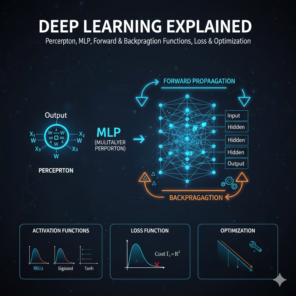
🔹 3. Perceptron — The Elementary Unit

A perceptron is the simplest artificial neuron. It receives inputs, multiplies each by a weight, adds a bias, and produces an output based on an activation function.

Equation:$$z = w_1x_1 + w_2x_2 + \cdots + w_nx_n + b$$z=w1​x1​+w2​x2​+⋯+wn​xn​+b $$\text{output} = f(z)$$output=f(z)

Where:

• $x_i$xi​ = input
• $w_i$wi​ = weight
• $b$b = bias
• $f$f = activation function (like sigmoid, ReLU, etc.)

Diagram — Perceptron:

 x1─►*w1
                 → Σ → f() → output
 x2─►*w2        + b

Here, each * input is weighted, summed, and then passed through a non-linear function.

📍 4. Single-Layer Perceptron — A Simple Network

This is the simplest neural network: inputs connect directly to the output neuron — no hidden layer.

x1 → 
       → Perceptron → y
x2 →

It can only learn linear relationships. That means it can solve problems like AND and OR but not XOR. The solution boundary is a straight line. This limitation led to deeper models.

🧠 5. Multi-Layer Perceptron (MLP) — Adding Depth

When you add one or more hidden layers, the network becomes a Multi-Layer Perceptron (MLP). This introduces non-linear decision boundaries and much greater learning power.

Input Layer → Hidden Layer(s) → Output Layer

Example with one hidden layer:

x1 ─► ◉ ─►
           ◉ ─► Output
x2 ─► ◉ ─►

More layers mean deeper representations — the network can learn more complex features step by step.

🔁 6. Forward Propagation — How Predictions Happen

Forward propagation is how the network processes data to make a prediction. Each layer multiplies the input by weights, adds bias, and applies an activation function.

General math for a neuron:$$a^{(l)} = f\left(W^{(l)}a^{(l-1)} + b^{(l)}\right)$$a(l)=f(W(l)a(l−1)+b(l))

Where:

• $a^{(l)}$a(l) = activation in layer $l$l
• $W^{(l)}$W(l), $b^{(l)}$b(l) = weights and biases
• $f()$f() = activation function

Diagram — Forward Pass:

Input → [Layer1] → [Layer2] → ... → Output

Each layer’s output becomes the next layer’s input, creating a chain of transformations that extract deeper features from data.

🔥 7. Activation Functions — Adding Non-Linearity

Without activation functions, a neural network would behave like a linear model regardless of depth. That’s why activations are critical!

Here are the most common ones:

🟢 Sigmoid

$$\sigma(x) = \frac{1}{1 + e^{-x}}$$σ(x)=1+e−x1​

Range: (0,1) — good for binary classification.

🔵 Tanh

$$\tanh(x) = \frac{e^x – e^{-x}}{e^x + e^{-x}}$$tanh(x)=ex+e−xex−e−x​

Range: (−1,1) — zero-centered.

🔶 ReLU (most popular)

$$\text{ReLU}(x) = \max(0, x)$$ReLU(x)=max(0,x)

Activates only positive values — fast and simple.

🟣 Leaky ReLU

Similar to ReLU but allows a tiny negative slope to avoid “dead neurons.”

🔻 Softmax

Transforms outputs into probabilities that sum to 1 — used in multi-class classification.

Activation Diagram (ASCII):

 x    sigmoid     tanh      ReLU
----   ─────    ─────–     ─────
-3     ~0.05     ~-0.995    0
 0     0.5       0          0
 3     ~0.95     ~0.995     3

📉 8. Loss Functions — How We Measure Error

A loss function tells us how far the network’s prediction is from the actual target. Minimizing loss is the goal of training.

Common loss functions:

📌 Regression

• Mean Squared Error (MSE):

$$\text{MSE} = \frac{1}{n}\sum (y_{\text{pred}} – y_{\text{true}})^2$$MSE=n1​∑(ypred​−ytrue​)2

📌 Classification

• Cross-Entropy Loss — measures difference between predicted probabilities and true classes.

Loss values drive the learning process — the higher the loss, the more the model needs to adjust.

🔄 9. Backpropagation — How Networks Learn

Backpropagation computes how the loss changes with respect to each weight using calculus’ chain rule, and then uses this gradient to update the weights.

Core idea (mathematically):$$\frac{\partial \text{Loss}}{\partial w} = \text{chain rule}$$∂w∂Loss​=chain rule

If the loss increases with respect to a weight, adjust the weight to reduce loss.

Visualization — Backpropagation:

           Error
             ↑
         [Output]
             ↑
   ←======== backpropagation
[layer 3] ← [layer 2] ← [layer 1]

Errors flow backward through the network, adjusting weights layer by layer.

⚙️ 10. Optimization — Gradient Descent & More

Once gradients are computed, we use an optimizer to update weights:$$w := w – \eta \cdot \frac{\partial \text{Loss}}{\partial w}$$w:=w−η⋅∂w∂Loss​

Where:

• $w$w = weight
• $\eta$η = learning rate

Common optimizers:

• Gradient Descent — update on full data
• Stochastic Gradient Descent (SGD) — update per data point
• Adam, RMSprop — adaptive learning rate methods

Optimizers control how quickly the network converges to a good solution.

📊 11. Putting It All Together — A Full Training Cycle

Here’s the complete training loop:

1. Forward propagation — compute predictions
2. Compute loss — how wrong are predictions?
3. Backpropagation — calculate gradients
4. Update weights — optimizer steps
5. Repeat — over many epochs until performance stabilizes

input → forward → loss → backward → update weights

This cycle is what makes deep learning work.

⭐ 12. Why Deep Learning Works So Well Today

Deep learning has transformed many fields because:

• It can learn raw features automatically, no hand-crafting needed.
• Modern GPUs enable fast training thanks to parallel linear algebra.
• Large datasets fuel deep models to generalize well.

This is why models like Convolutional Neural Networks and Transformers dominate modern AI.

🏁 Summary

Deep learning isn’t magic — it’s a mathematical and computational framework that:

✔ Learns hierarchical features
✔ Uses activation functions to model non-linearity
✔ Propagates error backward to update weights
✔ Optimizes performance via gradient descent

Deep learning represents one of the most significant advancements in artificial intelligence and machine learning in recent decades. At its core, deep learning is a subset of machine learning that leverages multi-layered neural networks to automatically learn representations and patterns from data without requiring manual feature engineering. These neural networks consist of interconnected layers of computational units — starting from simple processing units like the perceptron, and expanding into complex structures with many hidden layers that can extract increasingly abstract features from raw data.

We began our exploration by understanding the perceptron, the basic building block of all neural networks. A single-layer perceptron can only solve linearly separable problems due to its simple structure and lack of hidden processing units. By introducing one or more hidden layers — forming a multi-layer perceptron (MLP) — the networks gain the ability to capture non-linear and complex relationships in data, making them far more powerful and applicable to real-world tasks.

A major part of deep learning lies in how these networks learn. During forward propagation, input data is passed through the network, with each layer applying weights, biases, and activation functions to transform the data into a form suitable for prediction. The network’s prediction is then compared with the actual output using a loss function, which quantifies how far off the prediction is. The backpropagation algorithm then propagates this error backward through the network, allowing the model to adjust the weights and biases in a way that minimizes the loss over time.

Activation functions such as ReLU, sigmoid, and tanh introduce the necessary non-linear behavior into the network, enabling it to model complex patterns that a simple linear combination of inputs could never capture. Loss functions—like mean squared error for regression or cross-entropy for classification—serve as the objective measures that guide the optimization process. Optimization algorithms, including variants of gradient descent and adaptive methods like Adam and RMSprop, help update weights efficiently and steer the network toward better performance during training.

One of deep learning’s greatest strengths is its ability to automatically extract useful features from raw data, empowering it to tackle challenging tasks across domains such as computer vision, natural language processing, speech recognition, autonomous systems, and more. This ability stems from the hierarchical nature of neural networks — where early layers focus on basic features and deeper layers combine them into richer, higher-level concepts without explicit feature engineering.

However, deep learning also has its challenges. These models often require large volumes of labeled data, significant computational resources for training, and they are frequently described as black boxes due to their complexity and limited interpretability. Despite these challenges, innovations in computing power and training algorithms have made deep learning indispensable in modern AI systems.

In summary, deep learning is not merely a technique — it is a paradigm for learning from data that has reshaped the way machines understand and interact with the world. By uniting mathematical rigor, computational power, and rich architectures like perceptrons and multilayer networks, deep learning continues to push the boundaries of what intelligent systems can achieve. As research and technology advance, its impact will only grow, unlocking ever more sophisticated applications across industries and scientific fields.